Start a workspace in Verily Workbench
Categories:
Purpose: This document walks you through how to use basic features of Verily Workbench, including creating a workspace, loading data and analyzing it in a notebook.
Synopsis
The goal of this walkthrough is to show you what you need to know to achieve the following through the Verily Workbench web UI:
- Creating a workspace on your own
- Importing some data
- Accessing the data from a notebook running in a cloud app
- Performing basic data manipulation and analysis operations
- Saving and sharing your results
Note
This walkthrough is intentionally very concise. To learn more about each step and additional options that may be available, see the documentation referenced at each step.Prerequisites
Before you begin, you’ll need:
- A Workbench account
- To be a member of at least one pod. Each pod is linked to a cloud account used for billing, allowing you to perform operations that incur costs (i.e., creating workspaces, creating and running cloud apps, and storing data on the cloud).
Please contact support if you need a Workbench account or membership to a pod.
Finally, it's helpful, though not required, if you're familiar with basic JupyterLab notebook usage and R code.
Verily Workbench features
Let's get started with some of Workbench's key features.
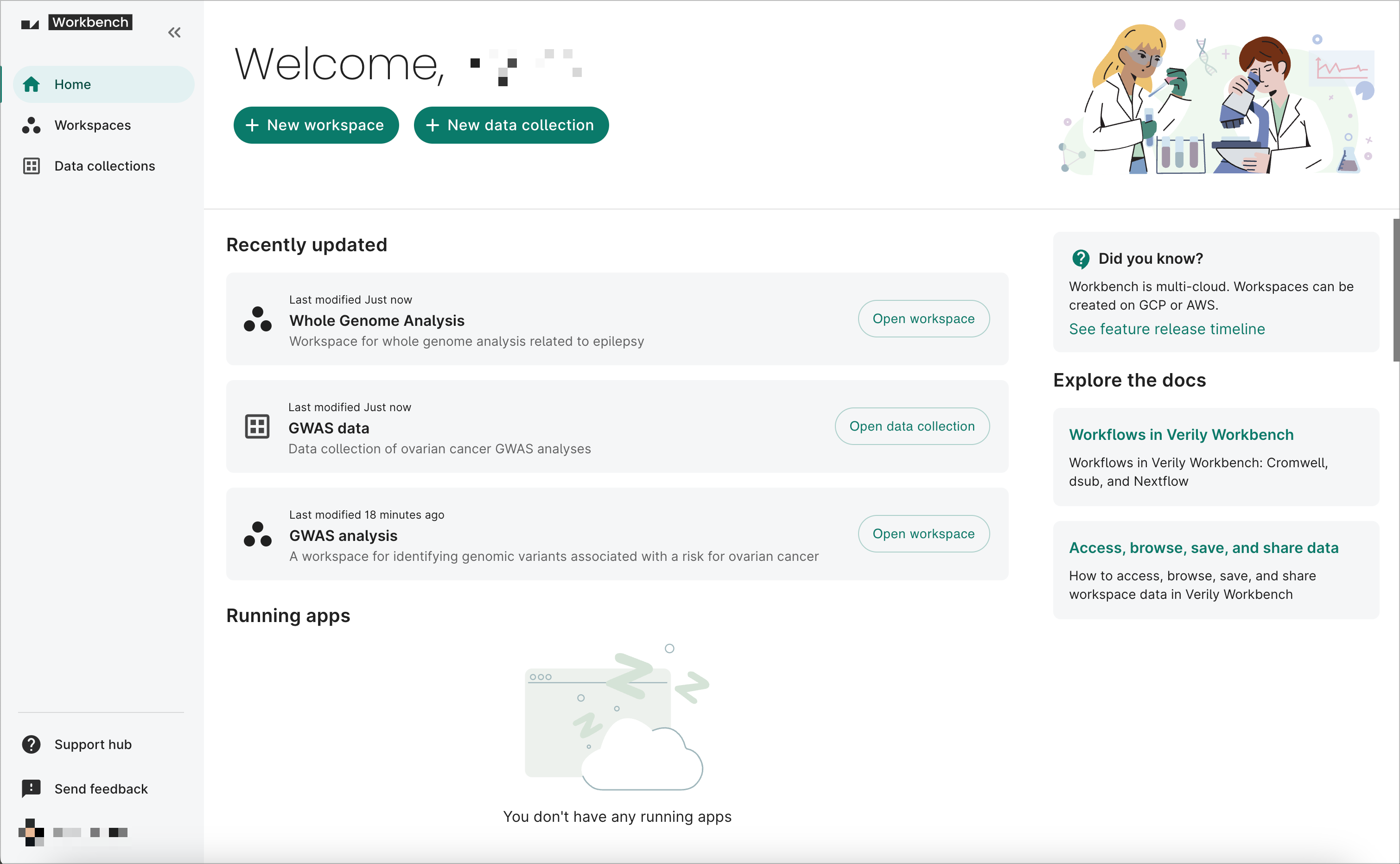
1. Explore the home page
The Workbench home page provides a quick overview of your recently updated workspaces and data collections. It also lets you create a new workspace or data collection, as well as view and stop any running apps.
You can also see helpful "Did you know?" tips and links to other Support hub documentation that will help you make the most out of Workbench.
2. Create a workspace
To create a workspace, follow the steps below:
- Navigate to the Workbench home page.
- Sign in using your registered email address.
- Click the + New workspace button on the welcome page. This will open the Create a new workspace dialog.
- Complete the three dialog screens. The workspace name and pod are the only fields that require your input; everything else is either optional or prefilled.
Be aware
You can't change the assigned pod once the workspace has been created.- Click the Create workspace button on the last screen. It should take less than a minute for the system to create your workspace. Once it’s done, your browser will load your new workspace’s overview page.
3. Add cloud resources to the workspace
The bucket resources you add to a workspace will be automounted to the file system of any workspace apps that you create.
To add storage resources to the workspace, follow the steps below:
3.1. Connect to a storage bucket containing data
First, you're going to connect an external cloud storage bucket to your workspace, which will make it easy to access data in that bucket from your workspace. This bucket will be treated as a referenced resource.
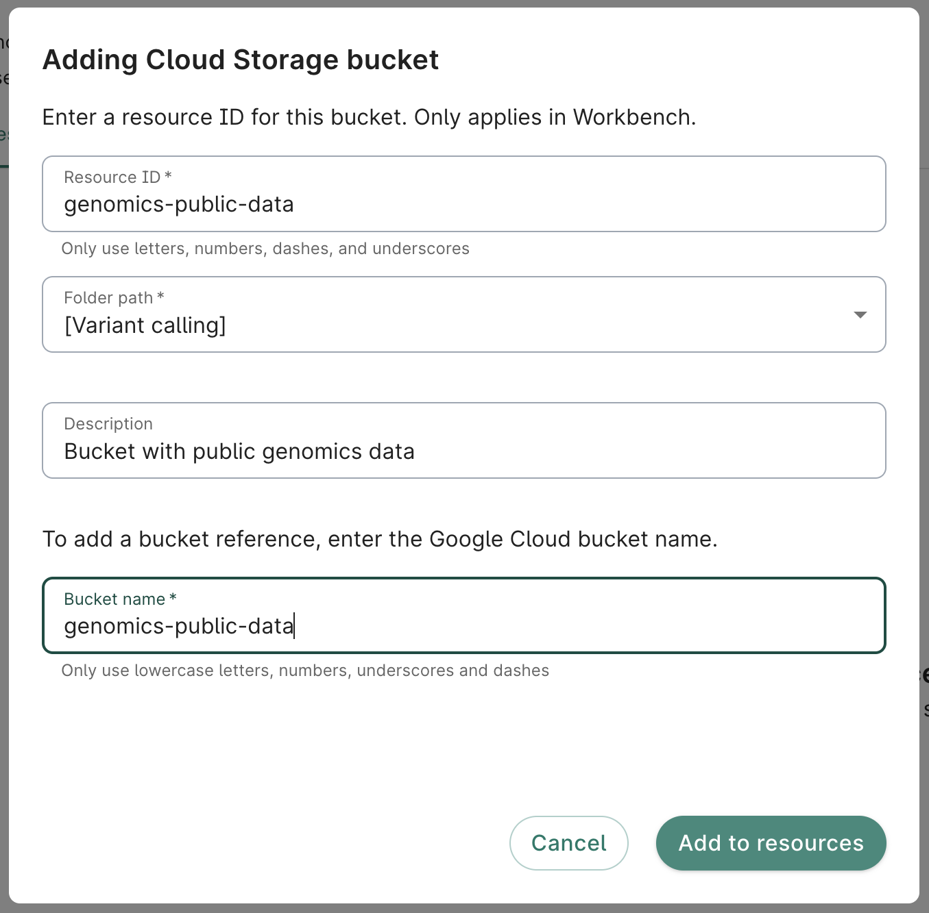
- Click on the Resources tab on your workspace page. Click on the + New resource button to open the menu of options, and select Reference Cloud Storage bucket to open the Adding Cloud Storage bucket dialog.
- Complete the form. The Resource ID, Folder path, and Bucket name fields are required. A description is not required, but recommended.
Note
Enter a memorable, descriptive ID in the Resource ID field. This is what will show up in your workspace's list of resources.In the Bucket name field, enter the name of the storage bucket you want to connect to. This should be an existing bucket that you already have access to. Do not include the
gs:// prefix. For testing purposes, you can use genomics-public-data, a public storage bucket that includes data from the 1000 Genomes Project.
- Click Add to resources. You should see the new resource appear immediately in the list of resources. You can test that you can access the bucket by clicking on the white Browse button in the information panel on the right of the Resources tab.
Note
You can also create a referenced resource to an object or folder in a Cloud Storage bucket, instead of pointing to the whole bucket. We'll see that in the example notebook referenced below.ℹ️ Data resource operations > Reference a storage bucket
3.2. Create a storage bucket for outputs
Now you have a workspace with data connected to it, but nowhere to store results of your analyses. Next, you're going to create a bucket that will be attached to the workspace itself, where you can store your outputs, as well as any other files and inputs that you might wish to associate with the workspace. This bucket will be treated as a controlled resource.
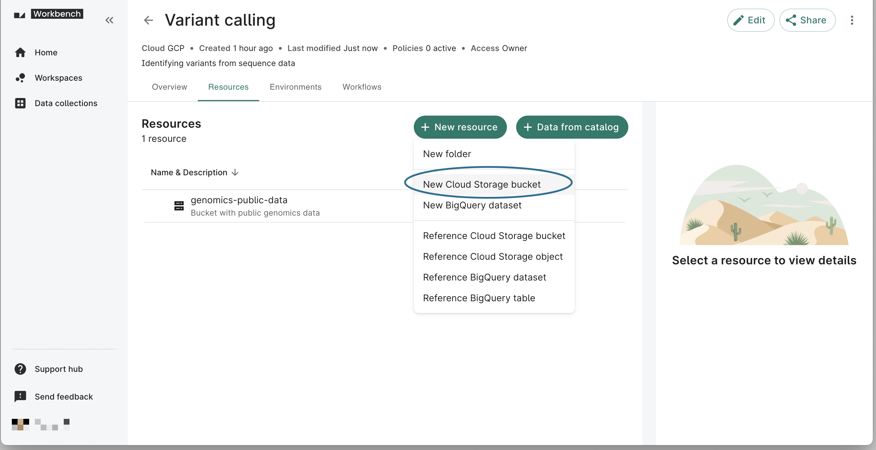
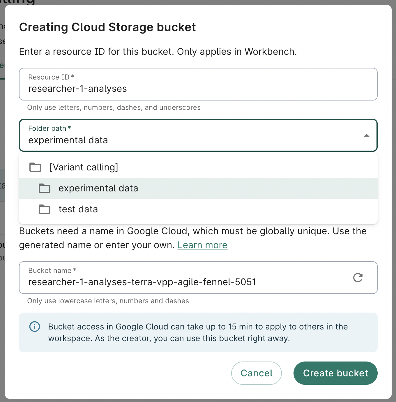
- Click on the Resources tab on your workspace page. Click on the + New resource button, then select New Cloud Storage bucket to open the Creating Cloud Storage bucket dialog.
- Complete the form. The Resource ID, Folder path, and Bucket name fields are required. A description is not required, but recommended.
Note
The Resource ID must be unique for the workspace.By default, the system will generate a bucket name (URI) for you, but you can change it. Note that you will not be able to change the name of your bucket later, and it has to be unique across all of Google Cloud.
- Click Create bucket. You should see the new resource appear immediately in the list of resources. You can confirm that you can access the bucket by clicking on the white Browse button on the right. Since it's brand new, the bucket should be empty.
Note: You can also create a referenced resource to an object or folder in a Cloud Storage bucket, instead of pointing to the whole bucket. We'll see that in the example notebook referenced below.
ℹ️ Data resource operations > Create a storage bucket
4. Create a reference to a Git repository
Follow the steps below to add a Git repository to your workspace's app(s):
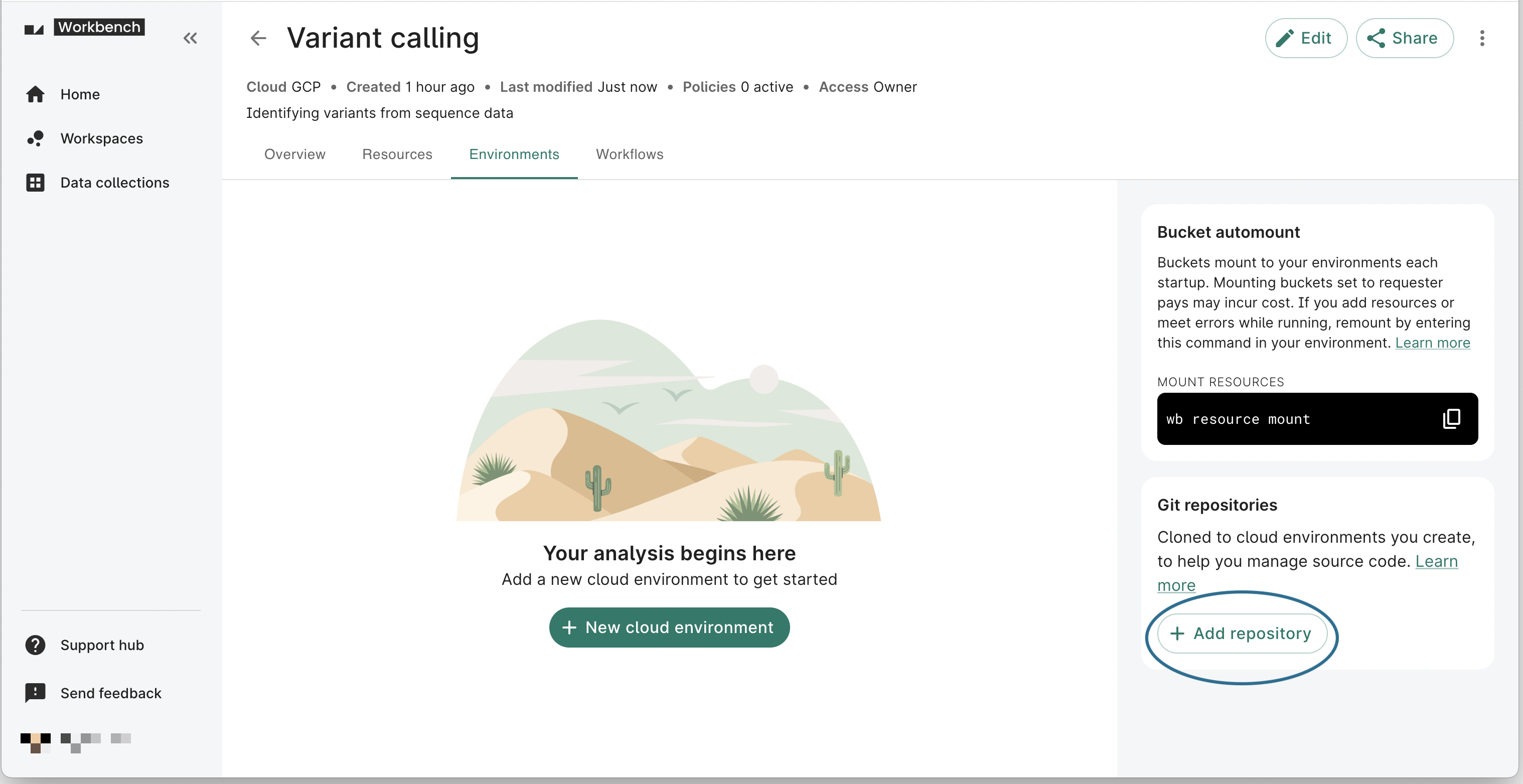
- Click on the Apps tab on your workspace page. In the Git repositories card on the right-hand side, click the + Add repository button to open the Adding Git repository dialog.
- Complete the form. The Name and Repository URL fields are required. A description is not required, but recommended.
For testing purposes, give it the Name
workbench-examplesand add this public repository as the Repository URL:https://github.com/verily-src/workbench-examples.git.
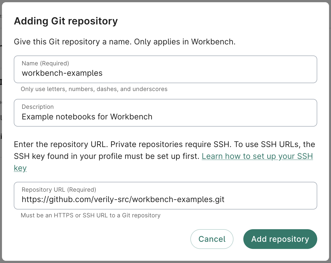
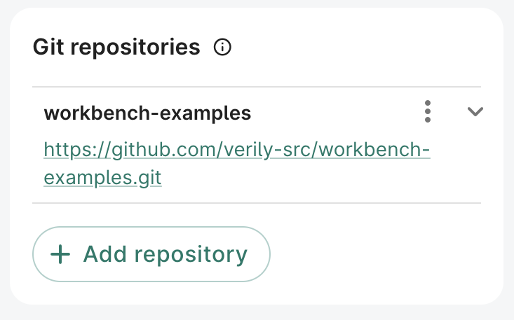
- Click Add repository. You'll now see the repo listed in the Git repositories card. This repo will be automatically cloned to any apps that you create in this workspace, which you'll do next.
5. Create an app
Next, you need to create and launch an app that will consist of a virtual machine (VM) with some preinstalled software and a local storage drive associated with it, called a persistent disk.
-
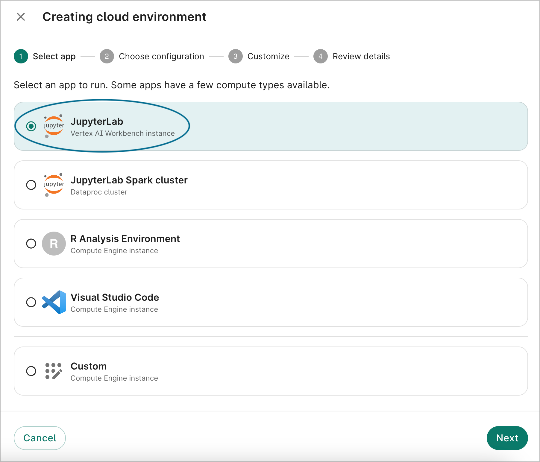
Click on the Apps tab on your workspace page. Click on the + New app instance button to open the Creating app dialog.
-
On the first dialog screen, select the JupyterLab option labeled Vertex AI Workbench instance. Click Next.
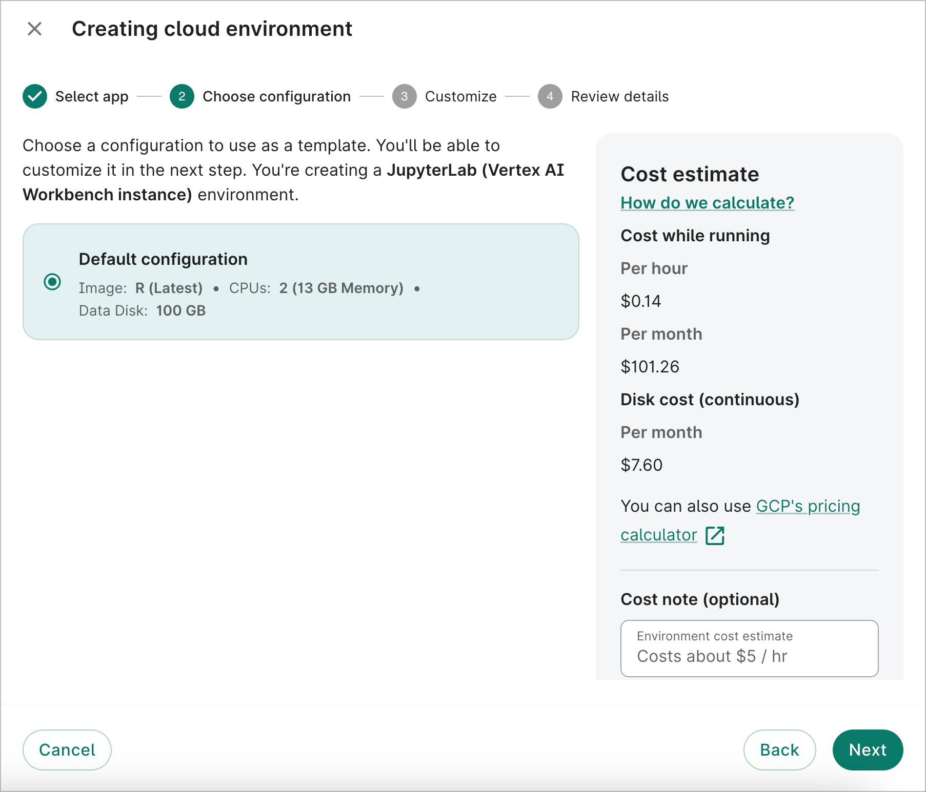
- On the second dialog screen, you'll be shown the default configuration. Click Next.
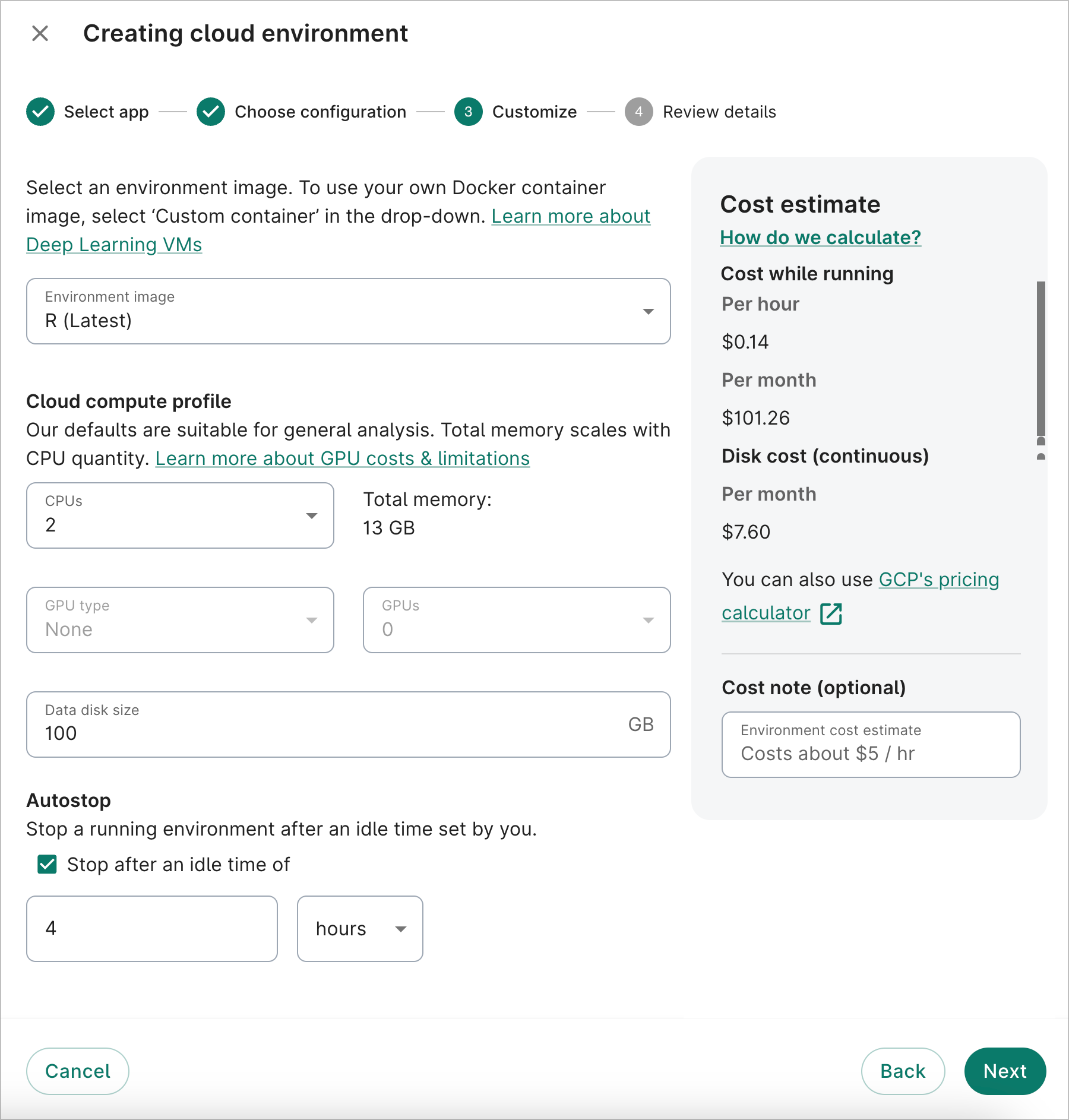
- On the third dialog screen, you can customize the app image type, the number of GPUs and CPUs (if applicable), the data disk size, and the autostop idle time. For this walkthrough, we'll select R (Latest) for the Image, since the analysis example below will use R code.
If you need more compute power, you can increase the number of CPUs to allocate; the memory allocated will scale accordingly. You can also attach GPUs to your app (if compatible with the selected app image). Keep in mind that the running cost of your app will scale with the computing resources allocated to it.
You can also change the default data disk size. 100 GB is recommended for most apps, but the size can range from 10 GB to 64,000 GB.
To help keep compute costs down, the autostop feature will automatically turn off your app after a certain time. An autostop idle time of four hours is enabled by default when you create an app. You can adjust the idle time to any value between 1 hour and 14 days, or opt out of autostop entirely. An app is considered “idle” when the app is not open in a browser, or if the CPU load on the VM is below 10% (e.g., there’s no background job running).
After finalizing your options, click Next.
- On the fourth dialog screen, give your app a memorable name in the Workbench ID field. Feel free to customize the Instance name or accept the one generated automatically by the system. A Description is not required, but recommended.
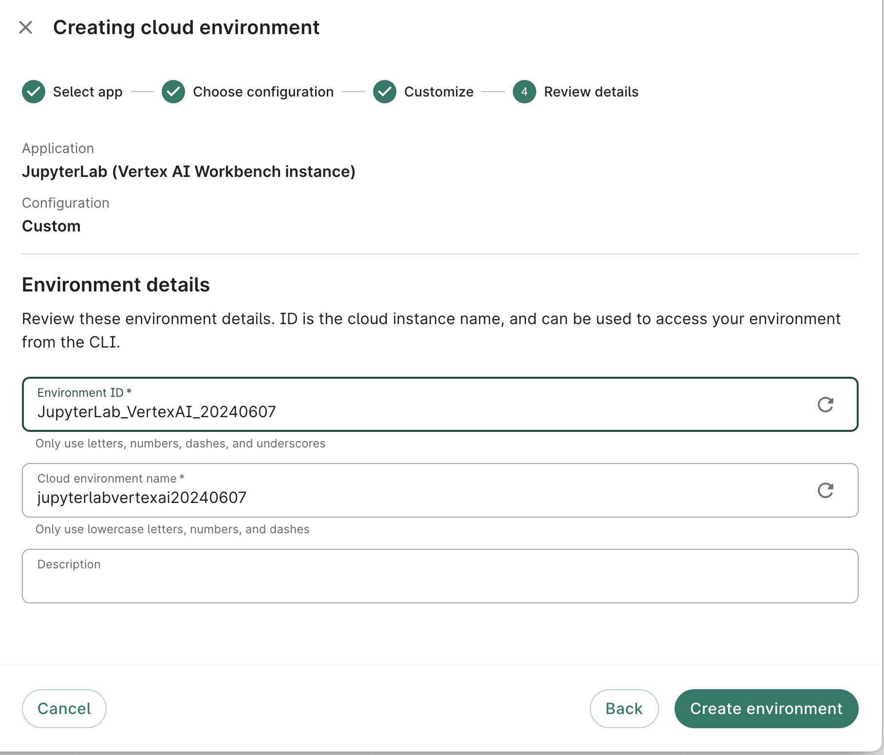
Click the Create app button. You should see a card for the new app appear in the Apps tab of your workspace, with a status indicator. It may take a few minutes for the system to get your app ready, depending on what resources you requested.
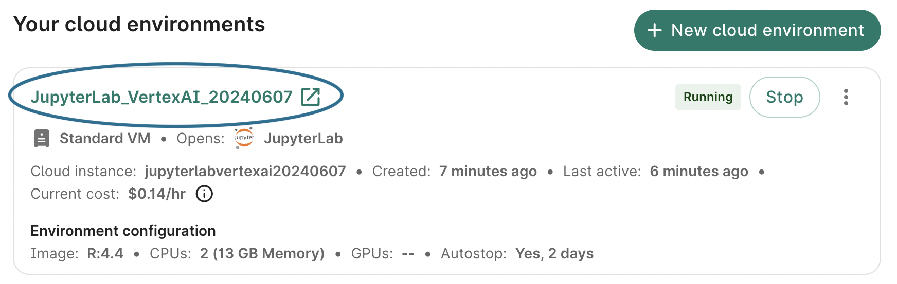
6. Open the Jupyter Notebook
Once your app is ready, the status indicator will turn green and display Running. Now, everything is set up for you to start working.
To start a JupyterLab session, click the Apps tab on your workspace page. Ensure the app is in Running status and click the Workbench ID of the notebook you'd like to access. This will open a JupyterLab session in a new browser window/tab, displaying the JupyterLab Launcher. It may take a minute to load.
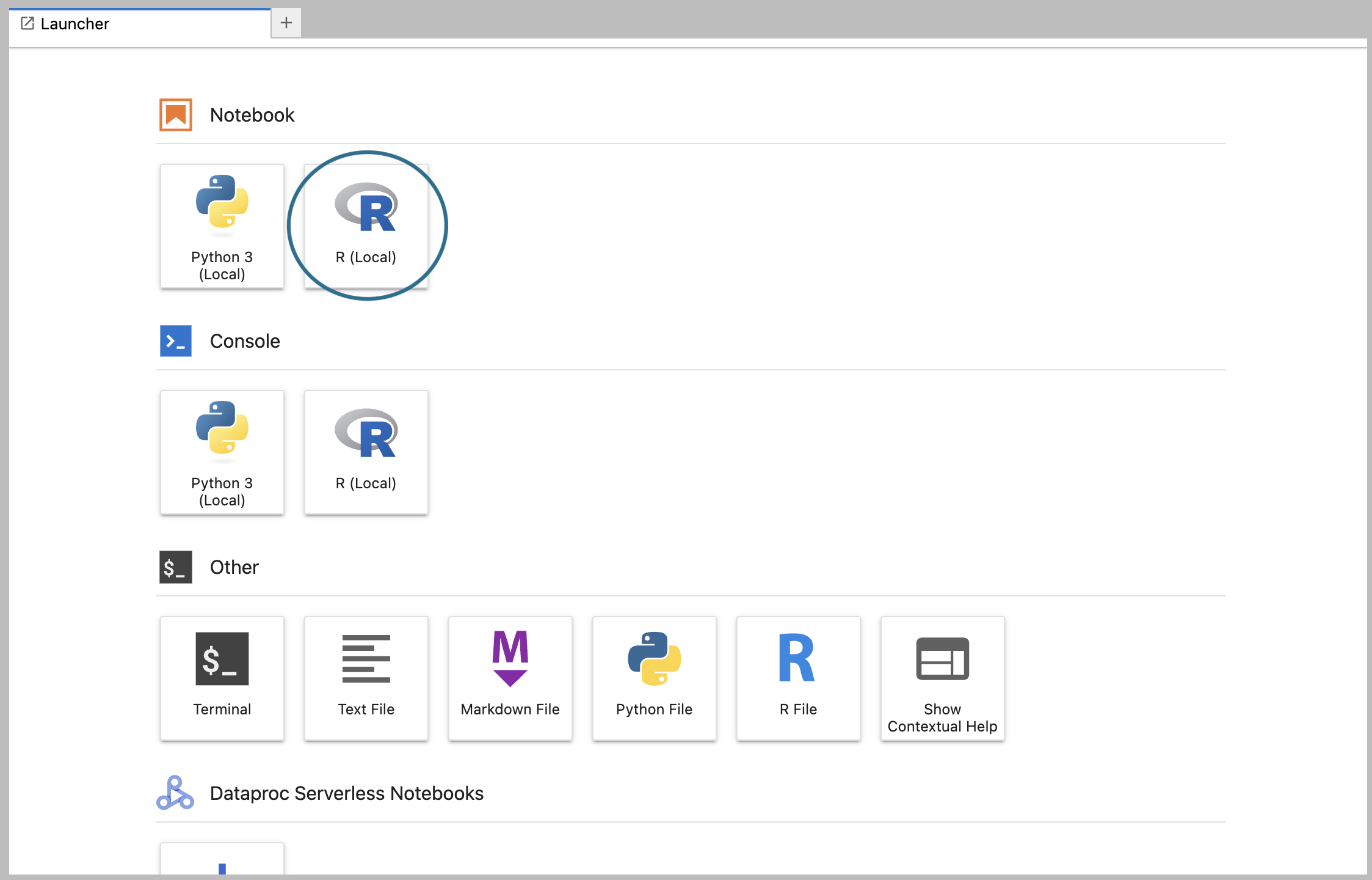
6.1. Open a new notebook
For the purposes of this walkthrough, we’re going to use example code written in R, so click on the R logo in the list of Notebook options. This will create a new R notebook file stored on your app's persistent disk, and open it for editing.
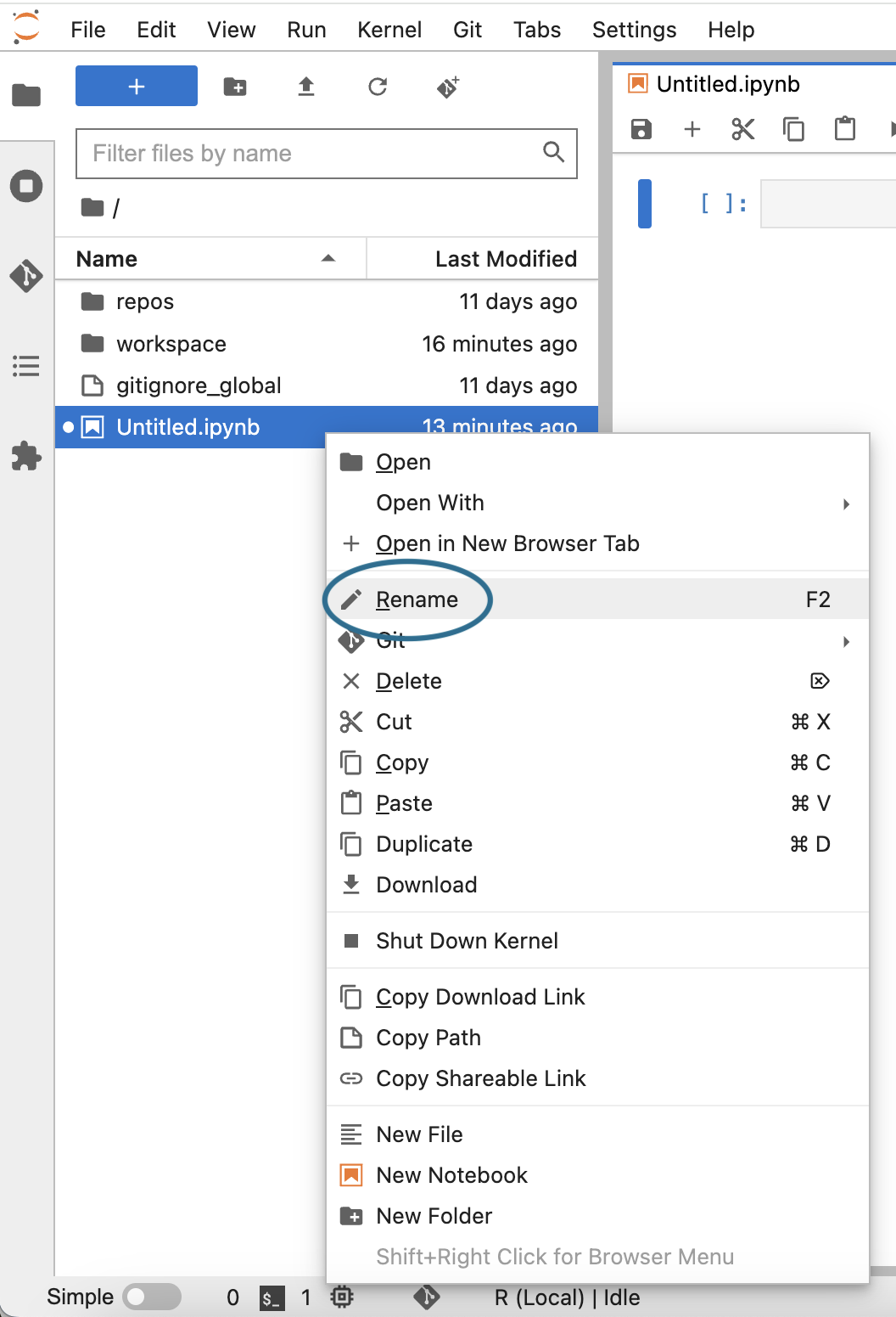
Give your new notebook a meaningful name. Right-click (or control-click) on the file name (which should be Untitled.ipynb) to open the contextual menu and select the Rename option.
You’ll find the file in the $HOME directory, which is displayed by default in the JupyterLab file explorer (left side panel). The file explorer allows you to access and organize any files stored on the persistent disk itself, and to access resources that are mounted to your app.
Now that you know how to create a new notebook, you won’t actually use it for the example below. Instead, you’ll open a pre-existing R notebook.
6.2. Open an existing notebook from an example repo
Next, open an existing notebook from the examples repo you added to the workspace in Step 3. This repo, workbench-examples, was automatically cloned to the JupyterLab server when you created your app. You will find it under repos in the file explorer (or /home/jupyter/repos in the Terminal).
In the file navigator, double-click repos, then workbench-examples, then 1kgenomes_examples. Double-click the R_1k_genomes.ipynb file to open it.
Note
If you did not add the GitHub repo previously, you can manually rungit clone https://github.com/verily-src/workbench-examples.git to add it to your notebook server.
7. Run an example notebook
To run the **R_1k_genomes.ipynb notebook that walks through the computation of principal components (PCA) of genomic variant data across one chromosome from 2,504 people from The 1000 enomes project, follow these steps below:
- Open the **R_1kgenomes.ipynb **notebook.
- Click the Run (▶) or Forward (⏩) button to run all the available commands on the notebook.
8. Turn down the app
Once you've finished your work and ensured everything is saved appropriately, you can close the JupyterLab browser window.
Return to your workspace's Apps tab and click the Stop button in the app card to turn down your app. This will immediately send the instruction to stop the app; there is no confirmation step. However, there may be a lag of a few seconds before the status is updated to Stopped in the graphical user interface. Alternatively, you can also stop your cloud environment in the Running apps section on the Workbench home page.
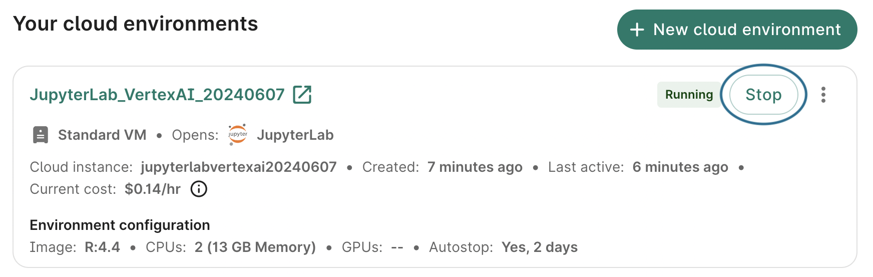
Be aware
Make sure you don't forget to stop your app because the cloud provider will continue to charge you as long as your app is running, even if it's not doing anything!ℹ️ Cloud app operations > Stop an app
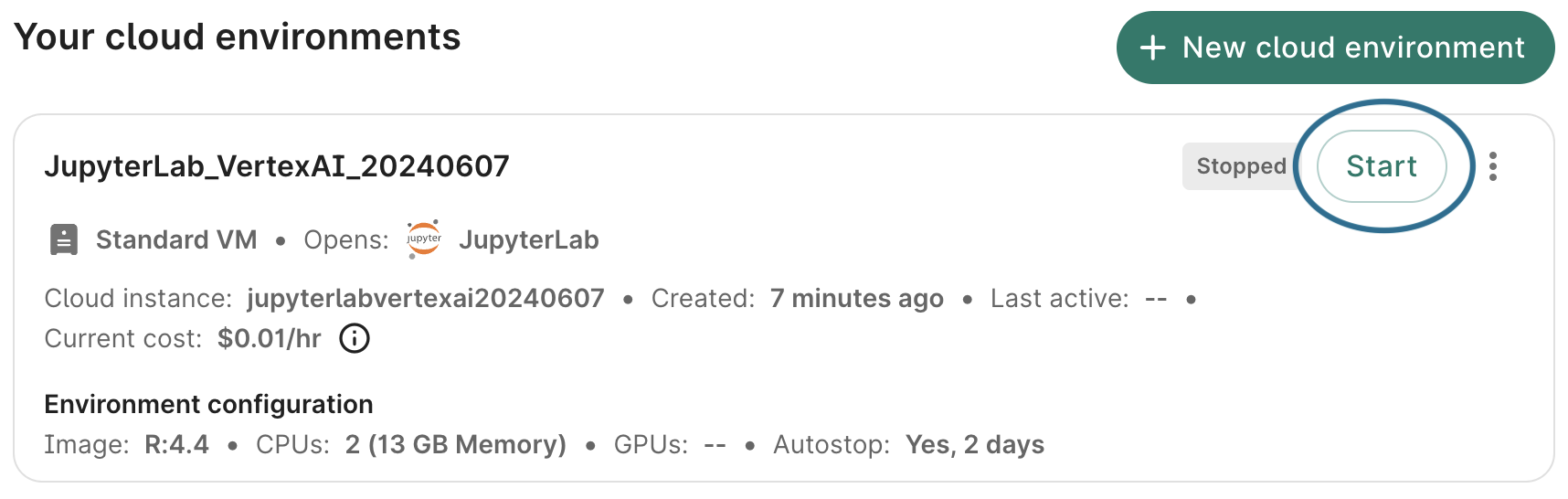
When you're ready to resume work, click the Start button in the app card. It may take a few minutes for an app to restart after being paused.
9. Delete the app
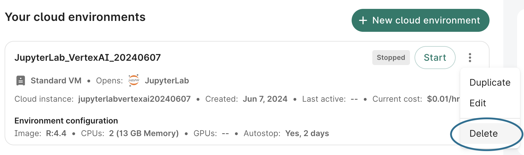
If you no longer need your app, you can delete it from the action menu of the app card:
- Click the Apps tab on your workspace page.
- Find the app you want to delete. Click the additional actions menu, which is represented by a "three-dot" icon in the top right corner of the app card.
- Click Delete. A dialog will open asking you to confirm deletion. Check the box and click the Delete app button.
Deletion of the app deletes its underlying disk as well. Therefore, make sure that you've preserved your work. You can do this by writing data and notebook files to your workspace bucket; this was shown in the example notebook. You can also commit work back to a GitHub repo, or download files to your local machine.
Last Modified: 12 November 2024